Building the A1 Differential Drive Robot

Recently I embarked on a project to build a differential drive robot from commercial parts. I intend to eventually use this platform for testing sensor fusion, localization, and mapping techniques. Initially, I built a platform to accomplish a simpler goal; to navigate along a user selected path.

System Design

Motor Selection and Mounting

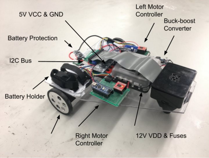
The robot was designed to navigate through an indoors environment at a speed of 40 cm/s which seemed reasonable. I was also concerned with selecting motors to achieve a smooth drive, especially when navigating over high friction surfaces like carpet. I searched for motors which could sustain around half a newton of force tangent to the wheel continuously. Often, one would consider continuous rotation servos in this case since they provide a gear motor with built-in closed-loop control. Continuous rotation servos which operate in this range can be quite expensive so I opted for a 110 rpm 5 kg cm DC gear motor. The motor came with a quadrature encoder that I used to provide feedback for a closed-loop control algorithm.

To mount the motor to the drive base, I created two mounting plates with a motor cage. This cage mounted to the bottom of the base plate with M3 screws. I also attached a passive caster to the base plate through a 3D printed offset. The base plate was made of 2 mm polycarbonate.

Electronics

To control the motors, I ended up using two Arduino Nanos because each motor requires two interrupt pins for each quadrature signal. A single Arduino Mega could be used to trigger interrupts but I had Arduino Nanos on hand. The Nanos interfaced with a TB6612FNG H-Bridge to provide speed control from a 12 V supply. A RPi 3B+ was used to perform the path calculations. The Nanos only have 2.5 kB of SRAM so the paths are stored on the RPi and fed over the I2C bus. Or at least, that was the idea. The current version stores the paths in flash. More on that later.

To power the robot, I used a three cell LiPo battery. This was connected to a BMS which provided over current and over discharge protection. The BMS output distributed power to each motor and a 5V buck-boost converter. Each was protected by a fuse.

Control Algorithms

The motion pipeline are composed of three stages:

1. Trajectories are generated on the RPi. These are provided to the motor controllers over the I2C bus.
2. The encoder signals are decoded and the position estimation is updated.
3. The trajectory and current motor position are used to calculate the input voltage for the motors.

Trajectory Generation

The paths are specified parametrically in the form <x(k), y(k)> This is transformed into a trajectory <x(t), y(t)> by time parametrizing it. This is a non-trivial problem since the rotational and forward velocities of a differential robot are intertwined: if motors are operating at their maximum velocity, an increase in the rotational velocity requires a decrease in the forward velocity. To plan a trajectory along a path, the maximum forward (tangent) velocity was calculated at each position k along the tangent path. This velocity limit varies with the curvature; the higher the curvature, the slower the robot can navigate along the path. Numerically, the forward velocity limit imposed by a single wheel (left or right) is proportional to the derivative of the tangent arc length with respect to the wheel arc length where the constant of proportionality is the max motor velocity. This provides a ceiling on the tangent velocity. The initial and final velocities along the path are known. This same process can be used to bound acceleration. The exact forward velocity transitions can be determined by a motion profile tuned to stay within the boundaries of these constraints. In my case, I used a simple trapezoidal profile. The tangent velocity function can be used to identify the position trajectories of each wheel. (In terms of path length.) These wheel position trajectories were fed to each motor controller.

Encoder Feedback

In order to provide accurate motion control, the system monitors the position of the motor and uses this information to make more informed estimates of the input voltage required to reach the target position. Quadrature encoders emit square waves on two channels A and B. Transitions in the signals A and B  encode changes in the motor position. For instance, when A transitions from low to high while B is low, this indicates that the motor has moved one section of an arc in the forward direction. If B made the transition before A, the encoder would move in the opposite direction. To decode the signal, the algorithm keeps a running tally of the number of arcs recorded. Each signal state is encoded in two bits. Following each state transition, the two bits representing the prior state and the two bits representing the current state query a lookup table containing the eight possible states. The counter is incremented or decremented according to the table entry. This maintains an accurate record of the encoder position. I've seen similar techniques in use elsewhere. In my case, this routine was triggered by a hardware interrupt. Triggering on interrupts ensures the algorithm doesn't miss a state transition while carrying out other control tasks.

Position Control

Armed with the trajectories, each motor controller was tasked with providing the correct input voltages to reach the designated positions. To accomplish this, it used feed forward motion control. Using this technique, the algorithm makes a crude initial guess at the input voltage. Then, it uses the known position, as obtained by the encoder, to correct this initial guess. A PID controller is used to make this correction. PID controllers are used commonly in industrial applications. Feed forward techniques, while less common, increase the responsiveness of the system to changes in the input position.

voltage = k_vf * v_setpoint + k_fa * a_setpoint + k_p * err + k_d * derr/dt

Known Issues

There are two main challenges with the current design. The first is that the 2 mm polycarbonate is flexible causing distortions in the width of the drive base. To mitigate this while testing, I added additional support to prevent the base board from flexing. A simple fix would be to combine both motor mounts into a single 3D print to add additional support. The second more significant issue is that the motors cause EMI on the I2C bus. I find it highly likely that this is due to high ground currents. I am currently experimenting with bus isolators to prevent the noise from affecting the bus.

Results

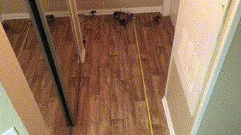
The result is a robot which can follow an input trajectory with surprising accuracy. I tested the robot against cosine, ellipse, and figure eight trajectories. In my testing, the robot generally deviated less than a centimeter along a five meter path.